Hysterical Squares
Rotation of rectangles in a grid using a general pattern for simulated hysteresis. This almost entirely derivative effort is a tweak code provided by @quantixed in their post Turn A Square: generative aRt. The incremental change here is to organize the calculated hysteresis as rectangles of line segments so they can be filled with colors using the ggplot2 library. Chose the viridis color palette here, it seemed to work nicely.
library(ggplot2)
library(viridis)
## Loading required package: viridisLite
Fill colors are based on the average shift in segments of a rectangle so the more twisted away from the grid the more the fill color will change.
The make_grid_art function will make grid art arguments define
- the number of squares in each dimension (xSize, ySize)
- grout defines the gap between squares (none = 0, max = 1)
- hFactor defines the amount of hysteresis (none = 0, max = 1, moderate = 10) For values above 1, larger values actually mean less shift
library(tidyverse)
## -- Attaching packages ------------------------------------------------------------------- tidyverse 1.3.0 --
## v tibble  3.0.3     v dplyr   1.0.2
## v tidyr   1.1.2     v stringr 1.4.0
## v readr   1.3.1     v forcats 0.5.0
## v purrr   0.3.4
## -- Conflicts ---------------------------------------------------------------------- tidyverse_conflicts() --
## x dplyr::filter() masks stats::filter()
## x dplyr::lag()    masks stats::lag()
library(viridis)

make_grid_art <- function(xSize, ySize, grout, hFactor) {
  xWave <- seq.int(1:xSize)
  yWave <- seq.int(1:ySize)
  axMin <- min(min(xWave) - 1,min(yWave) - 1)
  axMax <- max(max(xWave) + 1,max(yWave) + 1)
  nSquares <- length(xWave) * length(yWave)
  df <- data.frame()
  x <- 0
  halfGrout <- (1 - grout) / 2
  id_fact = max(xSize,ySize)
  for (i in seq_along(yWave)) {
    yCentre <- yWave[i]
    for (j in seq_along(xWave)) {
      if(hFactor < 1) {
        hyst <- rnorm(8, halfGrout, 0)
      }
      else {
        #shift for each line segment drawn standard distribution
        hyst <- rnorm(8, halfGrout, sin(x / (nSquares - 1) * pi) / hFactor)
      }
      xCentre <- xWave[j]
      id <- ((i-1)*id_fact) + j #id groups the segments for each rectangle
      edge_dist <- min(abs(i-1), abs(i-ySize),abs(j-1), abs(j-xSize))
      #using the mean of the tilt for edges as the color value
      fill <- mean(hyst) #fill color is the mean of hysteresis shift for segments
      lt <- c(xCentre - hyst[1],yCentre - hyst[2], id, fill, edge_dist)
      rt <- c(xCentre + hyst[3],yCentre - hyst[4], id, fill, edge_dist)
      rb <- c(xCentre + hyst[5],yCentre + hyst[6], id, fill, edge_dist)
      lb <- c(xCentre - hyst[7],yCentre + hyst[8], id, fill, edge_dist)
      df <- rbind(df, lt,rt,rb,lb)
      x <- x + 1
    }
  }
  names(df) <- c("x", "y", "id", "fill", "dist")
  p <- ggplot(df, aes(x=x, y=y, color=dist, fill=fill, group=id)) +
    geom_polygon(alpha=0.75) +
    scale_color_viridis(begin=0.35) +
    scale_fill_viridis() +
    theme_void() +
    guides(color=FALSE, fill=FALSE)
  print(p)
}
Then to create some variations on the parameters
# square grid with minimal hysteresis
make_grid_art(10,10,0.2,50)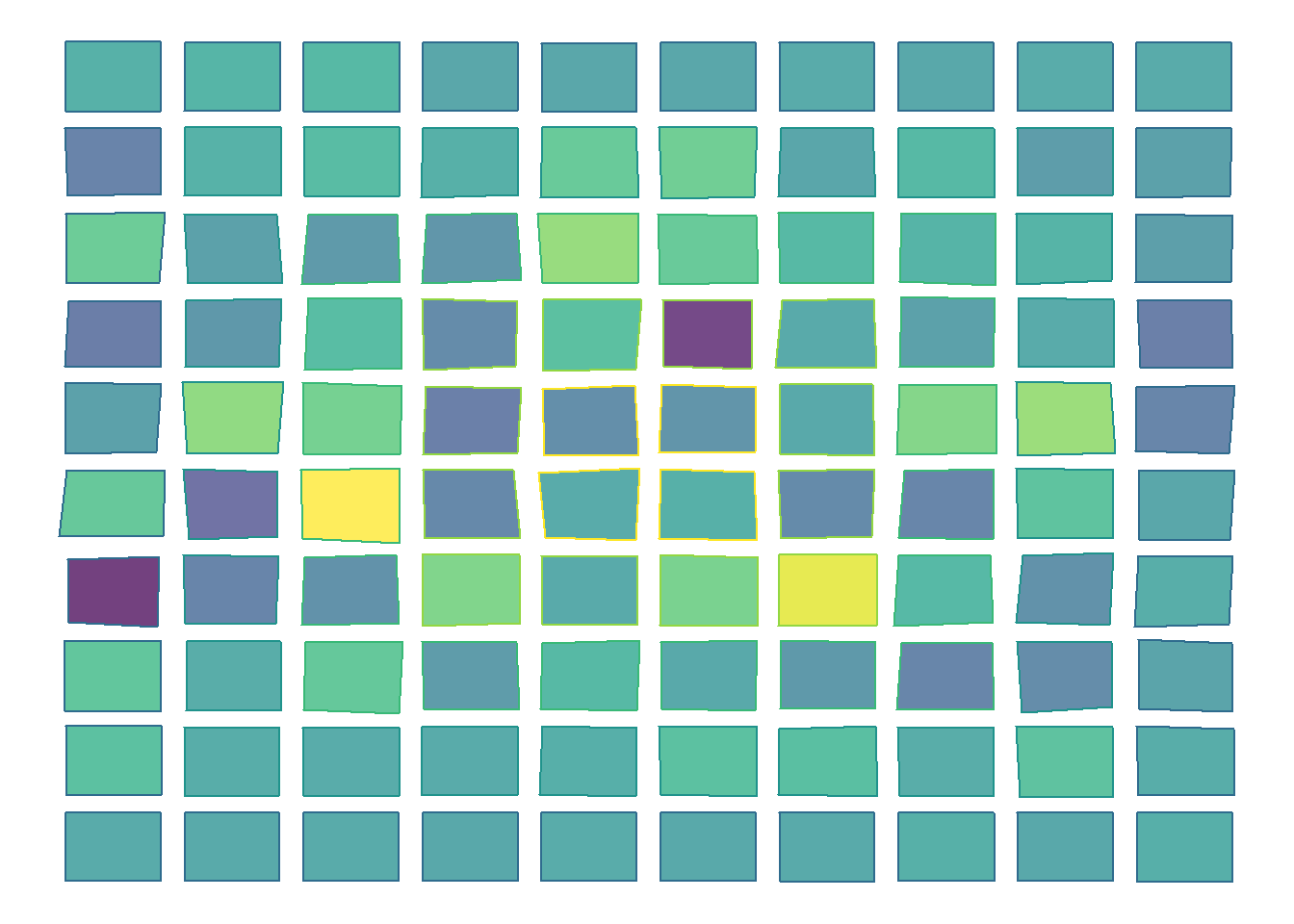
# square grid (more squares) more hysteresis
make_grid_art(20,20,0.02,10)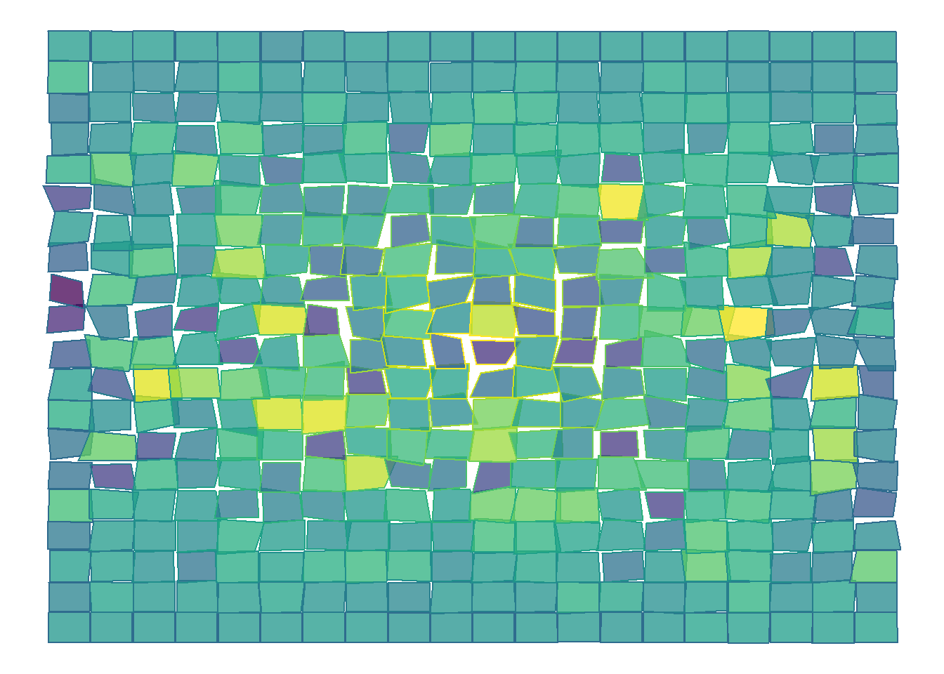
# rectangular grid same hysteresis
make_grid_art(25,15,0,10)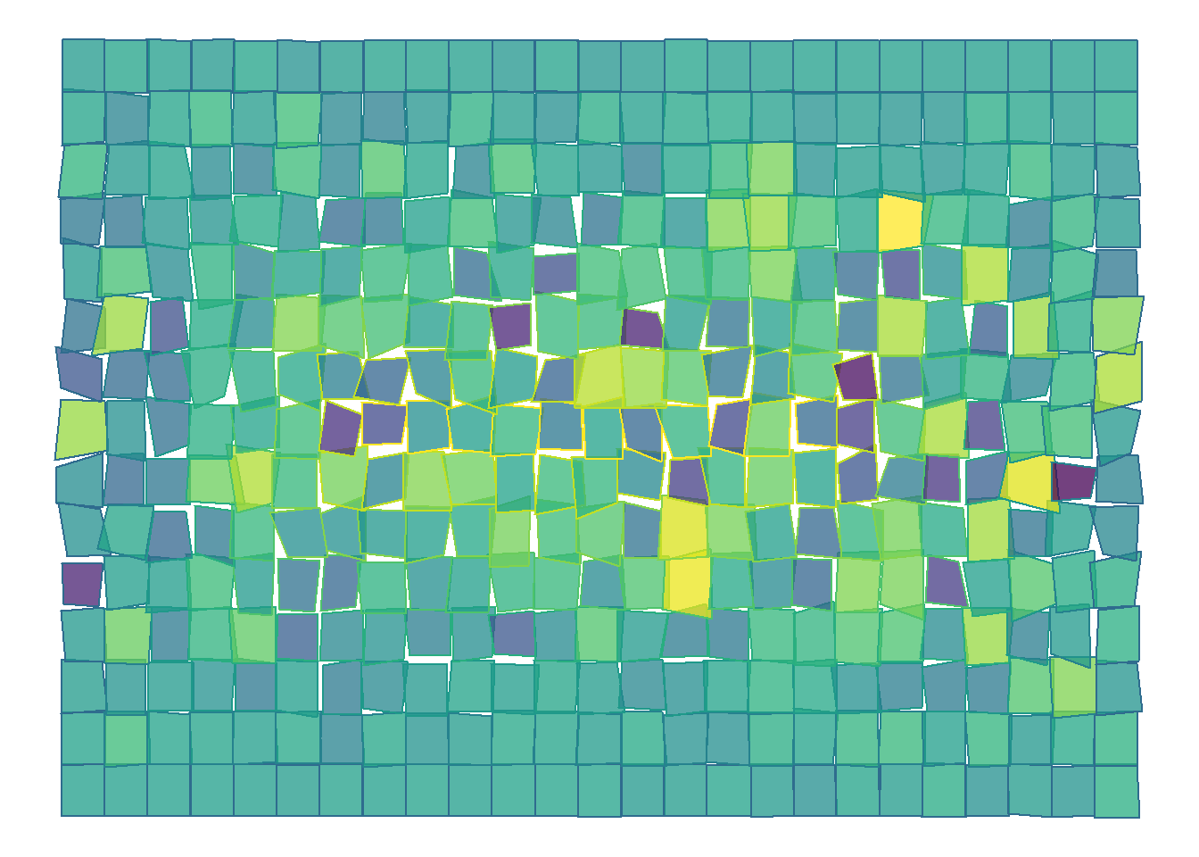
# same grid with no hysteresis
make_grid_art(25,15,0.08,0)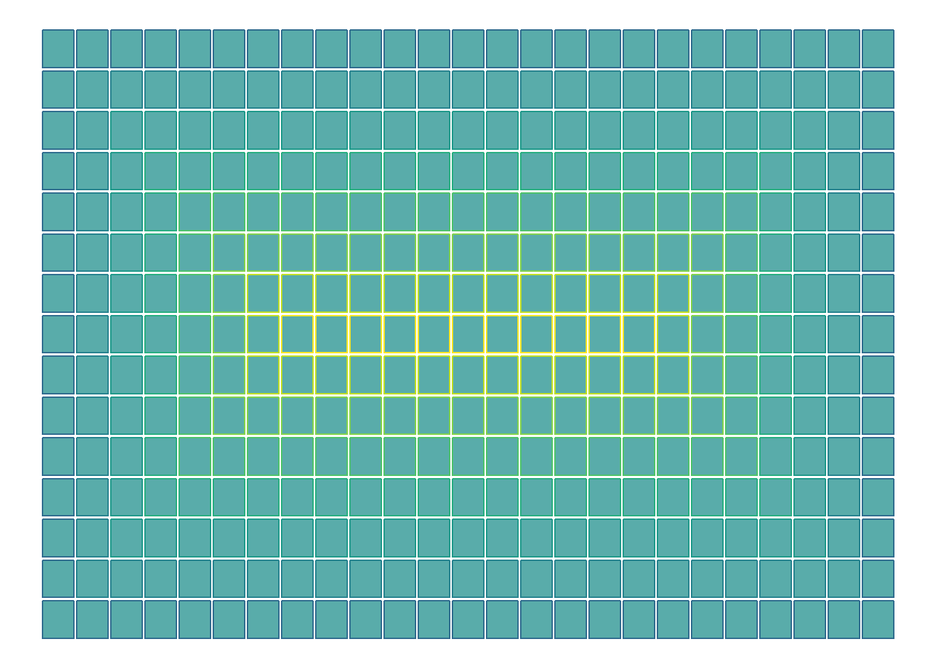
# square grid moderate hysteresis and no grout
make_grid_art(20,20,0,10)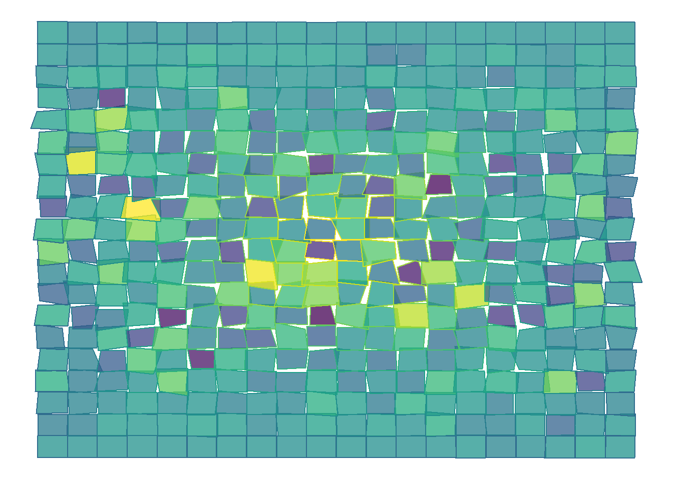
John Walker
I eat too much. Probably shouldn’t have lead with that.